Time-to-event (Survival)

Background

In healthcare, we deal with a lot of binary outcomes. Death yes/no, disease recurrence yes/no, for instance. These outcomes are often easily analysed using binary logistic regression via finalfit().

When the time taken for the outcome to occur is important, we need a different approach. For instance, in patients with cancer, the time taken until recurrence of the cancer is often just as important as the fact it has recurred.

Finalfit provides a number of functions to make these analyses easy to perform.

Installation

# Make sure finalfit is up-to-date 
install.packages("finalfit")

# For this vignette only, pre-specify table output
mykable = function(x){
    knitr::kable(x, row.names = FALSE, align = c("l", "l", "r", "r", "r", "r", "r", "r", "r"))
}

Dataset

We will use the classic “Survival from Malignant Melanoma” dataset which is included in the boot package. The data consist of measurements made on patients with malignant melanoma. Each patient had their tumour removed by surgery at the Department of Plastic Surgery, University Hospital of Odense, Denmark during the period 1962 to 1977.

We are interested in the association between tumour ulceration and survival after surgery.

Get data and check

library(finalfit)
melanoma = boot::melanoma #F1 here for help page with data dictionary
ff_glimpse(melanoma)
#> $Continuous
#>               label var_type   n missing_n missing_percent   mean     sd    min
#> time           time    <dbl> 205         0             0.0 2152.8 1122.1   10.0
#> status       status    <dbl> 205         0             0.0    1.8    0.6    1.0
#> sex             sex    <dbl> 205         0             0.0    0.4    0.5    0.0
#> age             age    <dbl> 205         0             0.0   52.5   16.7    4.0
#> year           year    <dbl> 205         0             0.0 1969.9    2.6 1962.0
#> thickness thickness    <dbl> 205         0             0.0    2.9    3.0    0.1
#> ulcer         ulcer    <dbl> 205         0             0.0    0.4    0.5    0.0
#>           quartile_25 median quartile_75    max
#> time           1525.0 2005.0      3042.0 5565.0
#> status            1.0    2.0         2.0    3.0
#> sex               0.0    0.0         1.0    1.0
#> age              42.0   54.0        65.0   95.0
#> year           1968.0 1970.0      1972.0 1977.0
#> thickness         1.0    1.9         3.6   17.4
#> ulcer             0.0    0.0         1.0    1.0
#> 
#> $Categorical
#> data frame with 0 columns and 205 rows

As can be seen, all variables are coded as numeric and some need recoding to factors. This is done below for for those we are interested in.

Death status

status is the the patients status at the end of the study.

1 indicates that they had died from melanoma;
2 indicates that they were still alive and;
3 indicates that they had died from causes unrelated to their melanoma.

There are three options for coding this.

Overall survival: considering all-cause mortality, comparing 2 (alive) with 1 (died melanoma)/3 (died other);
Cause-specific survival: considering disease-specific mortality comparing 2 (alive)/3 (died other) with 1 (died melanoma);
Competing risks: comparing 2 (alive) with 1 (died melanoma) accounting for 3 (died other); see more below.

Time and censoring

time is the number of days from surgery until either the occurrence of the event (death) or the last time the patient was known to be alive. For instance, if a patient had surgery and was seen to be well in a clinic 30 days later, but there had been no contact since, then the patient’s status would be considered 30 days. This patient is censored from the analysis at day 30, an important feature of time-to-event analyses.

Recode

library(dplyr)
#> 
#> Attaching package: 'dplyr'
#> The following objects are masked from 'package:stats':
#> 
#>     filter, lag
#> The following objects are masked from 'package:base':
#> 
#>     intersect, setdiff, setequal, union
library(forcats)
melanoma = melanoma %>%
  mutate(
    # Overall survival
    status_os = ifelse(status == 2, 0, # "still alive"
                                         1), # "died of melanoma" or "died of other causes"
    
    # Diease-specific survival
    status_dss = case_when(
        status == 2 ~ 0, # "still alive"
      status == 1 ~ 1, # "died of melanoma"
      TRUE ~  0),     # "died of other causes is censored"

    # Competing risks regression
    status_crr = case_when(
        status == 2 ~ 0, # "still alive"
      status == 1 ~ 1, # "died of melanoma"
      TRUE ~ 2),       # "died of other causes"
    
    # Label and recode other variables
    age = ff_label(age, "Age (years)"), # ff_label to make table friendly var labels
    thickness = ff_label(thickness, "Tumour thickness (mm)"), # ff_label to make table friendly var labels
    sex = factor(sex) %>% 
        fct_recode("Male" = "1", 
                             "Female" = "0") %>% 
        ff_label("Sex"),
    ulcer = factor(ulcer) %>% 
        fct_recode("No" = "0",
                             "Yes" = "1") %>% 
        ff_label("Ulcerated tumour")
  )

Kaplan-Meier survival estimator

We can use the excellent survival package to produce the Kaplan-Meier (KM) survival estimator. This is a non-parametric statistic used to estimate the survival function from time-to-event data.

library(survival)

survival_object = melanoma %$% 
    Surv(time, status_os)

# Explore:
head(survival_object) # + marks censoring, in this case "Alive"
#> [1]  10   30   35+  99  185  204

# Expressing time in years
survival_object = melanoma %$% 
    Surv(time/365, status_os)

KM analysis for whole cohort

Model

The survival object is the first step to performing univariable and multivariable survival analyses.

If you want to plot survival stratified by a single grouping variable, you can substitute “survival_object ~ 1” by “survival_object ~ factor”

# Overall survival in whole cohort
my_survfit = survfit(survival_object ~ 1, data = melanoma)
my_survfit # 205 patients, 71 events
#> Call: survfit(formula = survival_object ~ 1, data = melanoma)
#> 
#>        n events median 0.95LCL 0.95UCL
#> [1,] 205     71     NA    9.15      NA

Life table

A life table is the tabular form of a KM plot, which you may be familiar with. It shows survival as a proportion, together with confidence limits. The whole table is shown with, summary(my_survfit).

summary(my_survfit, times = c(0, 1, 2, 3, 4, 5))
#> Call: survfit(formula = survival_object ~ 1, data = melanoma)
#> 
#>  time n.risk n.event survival std.err lower 95% CI upper 95% CI
#>     0    205       0    1.000  0.0000        1.000        1.000
#>     1    193      11    0.946  0.0158        0.916        0.978
#>     2    183      10    0.897  0.0213        0.856        0.940
#>     3    167      16    0.819  0.0270        0.767        0.873
#>     4    160       7    0.784  0.0288        0.730        0.843
#>     5    122      10    0.732  0.0313        0.673        0.796
# 5 year overall survival is 73%

Kaplan Meier plot

We can plot survival curves using the finalfit wrapper for the package excellent package survminer. There are numerous options available on the help page. You should always include a number-at-risk table under these plots as it is essential for interpretation.

As can be seen, the probability of dying is much greater if the tumour was ulcerated, compared to those that were not ulcerated.

dependent_os = "Surv(time/365, status_os)"
explanatory = c("ulcer")

melanoma %>% 
    surv_plot(dependent_os, explanatory, pval = TRUE)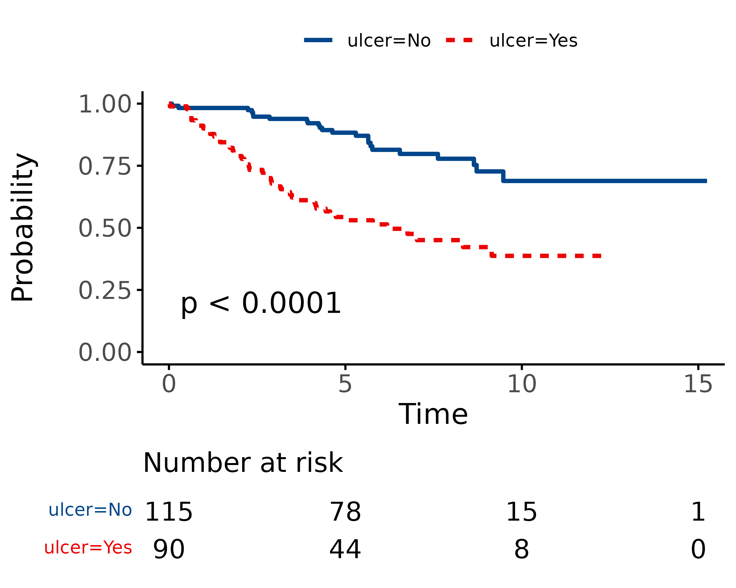

Cox-proportional hazards regression

CPH regression can be performed using the all-in-one finalfit() function. It produces a table containing counts (proportions) for factors, mean (SD) for continuous variables and a univariable and multivariable CPH regression.

Univariable and multivariable models

dependent_os = "Surv(time, status_os)"
dependent_dss = "Surv(time, status_dss)"
dependent_crr = "Surv(time, status_crr)"
explanatory = c("age", "sex", "thickness", "ulcer")

melanoma %>% 
    finalfit(dependent_os, explanatory) %>% 
    mykable() # for vignette only

Dependent: Surv(time, status_os)		all	HR (univariable)	HR (multivariable)
Age (years)	Mean (SD)	52.5 (16.7)	1.03 (1.01-1.05, p<0.001)	1.02 (1.01-1.04, p=0.005)
Sex	Female	126 (61.5)	-	-
	Male	79 (38.5)	1.93 (1.21-3.07, p=0.006)	1.51 (0.94-2.42, p=0.085)
Tumour thickness (mm)	Mean (SD)	2.9 (3.0)	1.16 (1.10-1.23, p<0.001)	1.10 (1.03-1.18, p=0.004)
Ulcerated tumour	No	115 (56.1)	-	-
	Yes	90 (43.9)	3.52 (2.14-5.80, p<0.001)	2.59 (1.53-4.38, p<0.001)

The labelling of the final table can be easily adjusted as desired.

melanoma %>% 
    finalfit(dependent_os, explanatory, add_dependent_label = FALSE) %>% 
    rename("Overall survival" = label) %>% 
    rename(" " = levels) %>% 
    rename("  " = all) %>% 
    mykable()

Overall survival			HR (univariable)	HR (multivariable)
Age (years)	Mean (SD)	52.5 (16.7)	1.03 (1.01-1.05, p<0.001)	1.02 (1.01-1.04, p=0.005)
Sex	Female	126 (61.5)	-	-
	Male	79 (38.5)	1.93 (1.21-3.07, p=0.006)	1.51 (0.94-2.42, p=0.085)
Tumour thickness (mm)	Mean (SD)	2.9 (3.0)	1.16 (1.10-1.23, p<0.001)	1.10 (1.03-1.18, p=0.004)
Ulcerated tumour	No	115 (56.1)	-	-
	Yes	90 (43.9)	3.52 (2.14-5.80, p<0.001)	2.59 (1.53-4.38, p<0.001)

Reduced model

If you are using a backwards selection approach or similar, a reduced model can be directly specified and compared. The full model can be kept or dropped.

explanatory_multi = c("age", "thickness", "ulcer")
melanoma %>% 
    finalfit(dependent_os, explanatory, explanatory_multi, keep_models = TRUE) %>% 
    mykable()

Dependent: Surv(time, status_os)		all	HR (univariable)	HR (multivariable full)	HR (multivariable)
Age (years)	Mean (SD)	52.5 (16.7)	1.03 (1.01-1.05, p<0.001)	1.02 (1.01-1.04, p=0.005)	1.02 (1.01-1.04, p=0.003)
Sex	Female	126 (61.5)	-	-	-
	Male	79 (38.5)	1.93 (1.21-3.07, p=0.006)	1.51 (0.94-2.42, p=0.085)	-
Tumour thickness (mm)	Mean (SD)	2.9 (3.0)	1.16 (1.10-1.23, p<0.001)	1.10 (1.03-1.18, p=0.004)	1.10 (1.03-1.18, p=0.003)
Ulcerated tumour	No	115 (56.1)	-	-	-
	Yes	90 (43.9)	3.52 (2.14-5.80, p<0.001)	2.59 (1.53-4.38, p<0.001)	2.72 (1.61-4.57, p<0.001)

Testing for proportional hazards

An assumption of CPH regression is that the hazard (think risk) associated with a particular variable does not change over time. For example, is the magnitude of the increase in risk of death associated with tumour ulceration the same in the early post-operative period as it is in later years?

The cox.zph() function from the survival package allows us to test this assumption for each variable. The plot of scaled Schoenfeld residuals should be a horizontal line. The included hypothesis test identifies whether the gradient differs from zero for each variable. No variable significantly differs from zero at the 5% significance level.

explanatory = c("age", "sex", "thickness", "ulcer", "year")
melanoma %>% 
    coxphmulti(dependent_os, explanatory) %>% 
    cox.zph() %>% 
    {zph_result <<- .} %>% 
    plot(var=5)

zph_result
#>           chisq df     p
#> age       2.067  1 0.151
#> sex       0.505  1 0.477
#> thickness 2.837  1 0.092
#> ulcer     4.325  1 0.038
#> year      0.451  1 0.502
#> GLOBAL    7.891  5 0.162

Stratified models

One approach to dealing with a violation of the proportional hazards assumption is to stratify by that variable. Including a strata() term will result in a separate baseline hazard function being fit for each level in the stratification variable. It will be no longer possible to make direct inference on the effect associated with that variable.

This can be incorporated directly into the explanatory variable list.

explanatory= c("age", "sex", "ulcer", "thickness", "strata(year)")
melanoma %>% 
    finalfit(dependent_os, explanatory) %>% 
    mykable()

Dependent: Surv(time, status_os)		all	HR (univariable)	HR (multivariable)
Age (years)	Mean (SD)	52.5 (16.7)	1.03 (1.01-1.05, p<0.001)	1.03 (1.01-1.05, p=0.002)
Sex	Female	126 (61.5)	-	-
	Male	79 (38.5)	1.93 (1.21-3.07, p=0.006)	1.75 (1.06-2.87, p=0.027)
Ulcerated tumour	No	115 (56.1)	-	-
	Yes	90 (43.9)	3.52 (2.14-5.80, p<0.001)	2.61 (1.47-4.63, p=0.001)
Tumour thickness (mm)	Mean (SD)	2.9 (3.0)	1.16 (1.10-1.23, p<0.001)	1.08 (1.01-1.16, p=0.027)
strata(year)			-	-

Correlated groups of observations

As a general rule, you should always try to account for any higher structure in your data within the model. For instance, patients may be clustered within particular hospitals.

There are two broad approaches to dealing with correlated groups of observations.

A cluster() term implies a generalised estimating equations (GEE) approach. Here, a standard CPH model is fitted but the standard errors of the estimated hazard ratios are adjusted to account for correlations.

A frailty() term implies a mixed effects model, where specific random effects term(s) are directly incorporated into the model.

Both approaches achieve the same goal in different ways. Volumes have been written on GEE vs mixed effects models. We favour the latter approach because of its flexibility and our preference for mixed effects modelling in generalised linear modelling. Note cluster() and frailty() terms cannot be combined in the same model.

# Simulate random hospital identifier
melanoma = melanoma %>% 
    mutate(hospital_id = c(rep(1:10, 20), rep(11, 5)))

# Cluster model
explanatory = c("age", "sex", "thickness", "ulcer", "cluster(hospital_id)")
melanoma %>% 
    finalfit(dependent_os, explanatory) %>% 
    mykable()

Dependent: Surv(time, status_os)		all	HR (univariable)	HR (multivariable)
Age (years)	Mean (SD)	52.5 (16.7)	1.03 (1.01-1.05, p<0.001)	1.02 (1.00-1.04, p=0.016)
Sex	Female	126 (61.5)	-	-
	Male	79 (38.5)	1.93 (1.21-3.07, p=0.006)	1.51 (1.10-2.08, p=0.011)
Tumour thickness (mm)	Mean (SD)	2.9 (3.0)	1.16 (1.10-1.23, p<0.001)	1.10 (1.04-1.17, p<0.001)
Ulcerated tumour	No	115 (56.1)	-	-
	Yes	90 (43.9)	3.52 (2.14-5.80, p<0.001)	2.59 (1.61-4.16, p<0.001)
cluster(hospital_id)			-	-

# Frailty model
explanatory = c("age", "sex", "thickness", "ulcer", "frailty(hospital_id)")
melanoma %>% 
    finalfit(dependent_os, explanatory) %>% 
    mykable()

Dependent: Surv(time, status_os)		all	HR (univariable)	HR (multivariable)
Age (years)	Mean (SD)	52.5 (16.7)	1.03 (1.01-1.05, p<0.001)	1.02 (1.01-1.04, p=0.005)
Sex	Female	126 (61.5)	-	-
	Male	79 (38.5)	1.93 (1.21-3.07, p=0.006)	1.51 (0.94-2.42, p=0.085)
Tumour thickness (mm)	Mean (SD)	2.9 (3.0)	1.16 (1.10-1.23, p<0.001)	1.10 (1.03-1.18, p=0.004)
Ulcerated tumour	No	115 (56.1)	-	-
	Yes	90 (43.9)	3.52 (2.14-5.80, p<0.001)	2.59 (1.53-4.38, p<0.001)
frailty(hospital_id)			-	-

The frailty() method here is being superseded by the coxme package, and we look forward to incorporating this in the future.

Hazard ratio plot

A plot of any of the above models can be easily produced.

melanoma %>% 
    hr_plot(dependent_os, explanatory)

#> Dependent variable is a survival object
#> Warning: Removed 3 rows containing missing values (`geom_errorbarh()`).
#> Warning: Removed 1 rows containing missing values (`geom_point()`).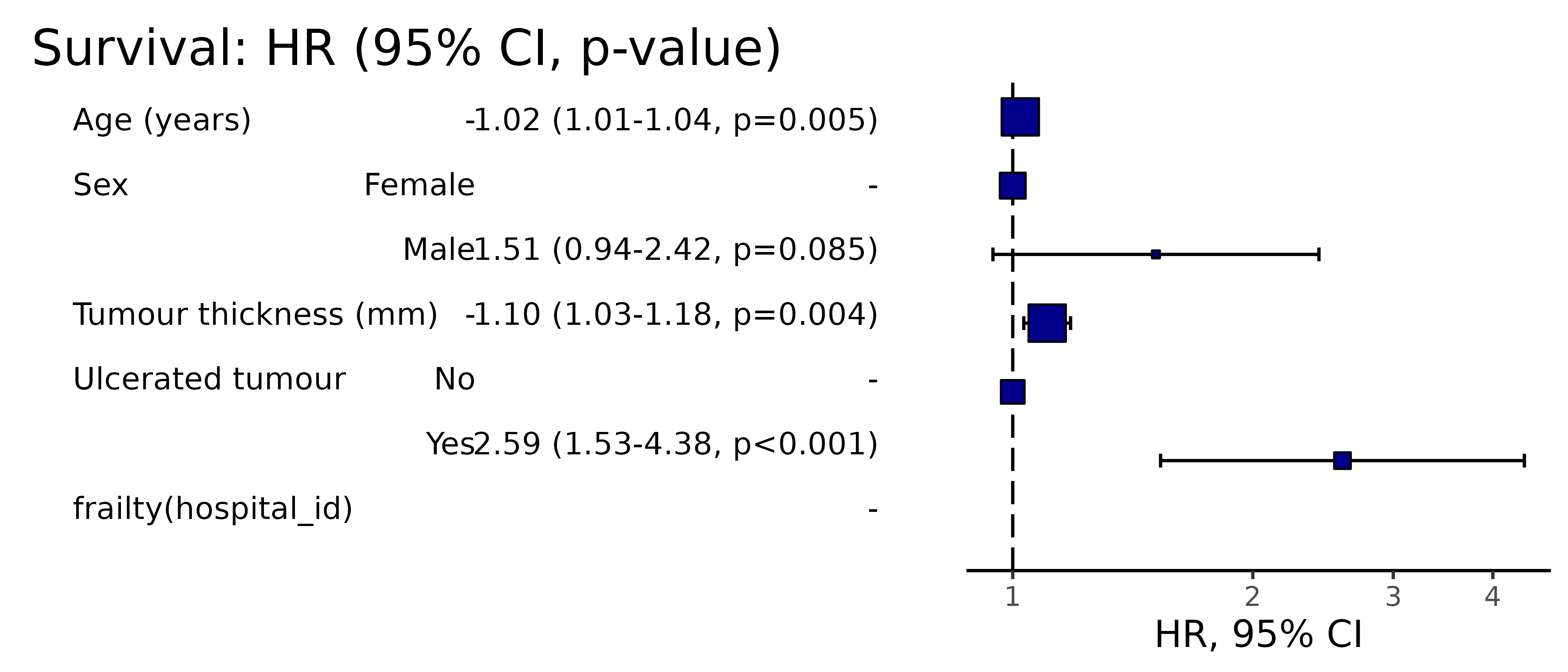

Competing risks regression

Competing-risks regression is an alternative to CPH regression. It can be useful if the outcome of interest may not be able to occur simply because something else (like death) has happened first. For instance, in our example it is obviously not possible for a patient to die from melanoma if they have died from another disease first. By simply looking at cause-specific mortality (deaths from melanoma) and considering other deaths as censored, bias may result in estimates of the influence of predictors.

The approach by Fine and Gray is one option for dealing with this. It is implemented in the package cmprsk. The crr() syntax differs from survival::coxph() but finalfit brings these together.

It uses the finalfit::ff_merge() function, which can join any number of models together.

explanatory = c("age", "sex", "thickness", "ulcer")
dependent_dss = "Surv(time, status_dss)"
dependent_crr = "Surv(time, status_crr)"

melanoma %>%
    
    # Summary table
  summary_factorlist(dependent_dss, explanatory, column = TRUE, fit_id = TRUE) %>%
    
    # CPH univariable
      ff_merge(
    melanoma %>%
      coxphmulti(dependent_dss, explanatory) %>%
      fit2df(estimate_suffix = " (DSS CPH univariable)")
    ) %>%
    
    # CPH multivariable
  ff_merge(
    melanoma %>%
      coxphmulti(dependent_dss, explanatory) %>%
      fit2df(estimate_suffix = " (DSS CPH multivariable)")
    ) %>%
    
    # Fine and Gray competing risks regression
  ff_merge(
    melanoma %>%
      crrmulti(dependent_crr, explanatory) %>%
      fit2df(estimate_suffix = " (competing risks multivariable)")
    ) %>%
    

  select(-fit_id, -index) %>%
  dependent_label(melanoma, "Survival") %>% 
    mykable()
#> Dependent variable is a survival object

Dependent: Survival		all	HR (DSS CPH univariable)	HR (DSS CPH multivariable)	HR (competing risks multivariable)
Age (years)	Mean (SD)	52.5 (16.7)	1.01 (1.00-1.03, p=0.141)	1.01 (1.00-1.03, p=0.141)	1.01 (0.99-1.02, p=0.520)
Sex	Female	126 (61.5)	-	-	-
	Male	79 (38.5)	1.54 (0.91-2.60, p=0.106)	1.54 (0.91-2.60, p=0.106)	1.50 (0.87-2.57, p=0.140)
Tumour thickness (mm)	Mean (SD)	2.9 (3.0)	1.12 (1.04-1.20, p=0.004)	1.12 (1.04-1.20, p=0.004)	1.09 (1.01-1.18, p=0.019)
Ulcerated tumour	No	115 (56.1)	-	-	-
	Yes	90 (43.9)	3.20 (1.75-5.88, p<0.001)	3.20 (1.75-5.88, p<0.001)	3.09 (1.71-5.60, p<0.001)

Summary

So here we have various aspects of time-to-event analysis which is commonly used when looking at survival. There are many other applications, some which may not be obvious: for instance we use CPH for modelling length of stay in in hospital.

Stratification can be used to deal with non-proportional hazards in a particular variable.

Hierarchical structure in your data can be accommodated with cluster or frailty (random effects) terms.

Competing risks regression may be useful if your outcome is in competition with another, such as all-cause death, but is currently limited in its ability to accommodate hierarchical structures.

Ewen Harrison