finalfit makes it easy to export final results tables
and plots from RStudio to Microsoft Word and PDF.
Make sure you are on the most up-to-date version of finalfit.
install.packages("finalfit")What follows is for demonstration purposes and is not meant to illustrate model building. We will ask, does a particular characteristic of a tumour (differentiation) predict 5-year survival?
Explore data
First explore variable of interest (exposure) by making it the dependent.
library(finalfit)
library(dplyr)

dependent = "differ.factor"

# Specify explanatory variables of interest
explanatory = c("age", "sex.factor",
  "extent.factor", "obstruct.factor",
  "nodes")
Note this useful alternative way of specifying explanatory variable lists:
colon_s %>%
  select(age, sex.factor, extent.factor, obstruct.factor, nodes) %>%
  names() -> explanatory
Check data.
colon_s %>%
  ff_glimpse(dependent, explanatory)
#> $Continuous
#>             label var_type   n missing_n missing_percent mean   sd  min
#> age   Age (years)    <dbl> 929         0             0.0 59.8 11.9 18.0
#> nodes       nodes    <dbl> 911        18             1.9  3.7  3.6  0.0
#>       quartile_25 median quartile_75  max
#> age          53.0   61.0        69.0 85.0
#> nodes         1.0    2.0         5.0 33.0
#>
#> $Categorical
#>                            label var_type   n missing_n missing_percent
#> differ.factor    Differentiation    <fct> 906        23             2.5
#> sex.factor                   Sex    <fct> 929         0             0.0
#> extent.factor   Extent of spread    <fct> 929         0             0.0
#> obstruct.factor      Obstruction    <fct> 908        21             2.3
#>                 levels_n
#> differ.factor          3
#> sex.factor             2
#> extent.factor          4
#> obstruct.factor        2
#>                                                                              levels
#> differ.factor                               "Well", "Moderate", "Poor", "(Missing)"
#> sex.factor                                            "Female", "Male", "(Missing)"
#> extent.factor   "Submucosa", "Muscle", "Serosa", "Adjacent structures", "(Missing)"
#> obstruct.factor                                            "No", "Yes", "(Missing)"
#>                     levels_count         levels_percent
#> differ.factor   93, 663, 150, 23 10.0, 71.4, 16.1,  2.5
#> sex.factor              445, 484                 48, 52
#> extent.factor   21, 106, 759, 43  2.3, 11.4, 81.7,  4.6
#> obstruct.factor     732, 176, 21       78.8, 18.9,  2.3
Demographics table
Look at associations between our exposure and other explanatory variables. Include missing data.
colon_s %>%
  summary_factorlist(dependent, explanatory,
p=TRUE, na_include=TRUE)| label | levels | Well | Moderate | Poor | p |
|---|---|---|---|---|---|
| Age (years) | Mean (SD) | 60.2 (12.8) | 59.9 (11.7) | 59.0 (12.8) | 0.644 |
| Sex | Female | 51 (54.8) | 314 (47.4) | 73 (48.7) | 0.400 |
| Male | 42 (45.2) | 349 (52.6) | 77 (51.3) | ||
| (Missing) | 0 (0.0) | 0 (0.0) | 0 (0.0) | ||
| Extent of spread | Submucosa | 5 (5.4) | 12 (1.8) | 3 (2.0) | 0.081 |
| Muscle | 12 (12.9) | 78 (11.8) | 12 (8.0) | ||
| Serosa | 76 (81.7) | 542 (81.7) | 127 (84.7) | ||
| Adjacent structures | 0 (0.0) | 31 (4.7) | 8 (5.3) | ||
| (Missing) | 0 (0.0) | 0 (0.0) | 0 (0.0) | ||
| Obstruction | No | 69 (74.2) | 531 (80.1) | 114 (76.0) | 0.655 |
| Yes | 19 (20.4) | 122 (18.4) | 31 (20.7) | ||
| (Missing) | 5 (5.4) | 10 (1.5) | 5 (3.3) | ||
| nodes | Mean (SD) | 2.7 (2.2) | 3.6 (3.4) | 4.7 (4.4) | <0.001 |
Note missing data in obstruct.factor. See a full
description of options in the forthcoming missing data vignette.
We will drop this variable for now. Also see that nodes has not been labelled. There are small numbers in some variables generating chisq.test warnings (predicted less than 5 in any cell). Generate final table.
explanatory = c("age", "sex.factor",
  "extent.factor", "nodes")

colon_s %>%
    mutate(
        nodes = ff_label(nodes, "Lymph nodes involved")
    ) %>%
  summary_factorlist(dependent, explanatory,
    p=TRUE, na_include=TRUE,
    add_dependent_label=TRUE) -> table 1
table1| Dependent: Differentiation | Well | Moderate | Poor | p | |
|---|---|---|---|---|---|
| Age (years) | Mean (SD) | 60.2 (12.8) | 59.9 (11.7) | 59.0 (12.8) | 0.644 |
| Sex | Female | 51 (54.8) | 314 (47.4) | 73 (48.7) | 0.400 |
| Male | 42 (45.2) | 349 (52.6) | 77 (51.3) | ||
| (Missing) | 0 (0.0) | 0 (0.0) | 0 (0.0) | ||
| Extent of spread | Submucosa | 5 (5.4) | 12 (1.8) | 3 (2.0) | 0.081 |
| Muscle | 12 (12.9) | 78 (11.8) | 12 (8.0) | ||
| Serosa | 76 (81.7) | 542 (81.7) | 127 (84.7) | ||
| Adjacent structures | 0 (0.0) | 31 (4.7) | 8 (5.3) | ||
| (Missing) | 0 (0.0) | 0 (0.0) | 0 (0.0) | ||
| Lymph nodes involved | Mean (SD) | 2.7 (2.2) | 3.6 (3.4) | 4.7 (4.4) | <0.001 |
Logistic regression table
Now examine explanatory variables against outcome. Check plot runs ok.
explanatory = c("age", "sex.factor",
  "extent.factor", "nodes", "differ.factor")
dependent = "mort_5yr"
colon_s %>%
  finalfit(dependent, explanatory,
  dependent_label_prefix = "") -> table2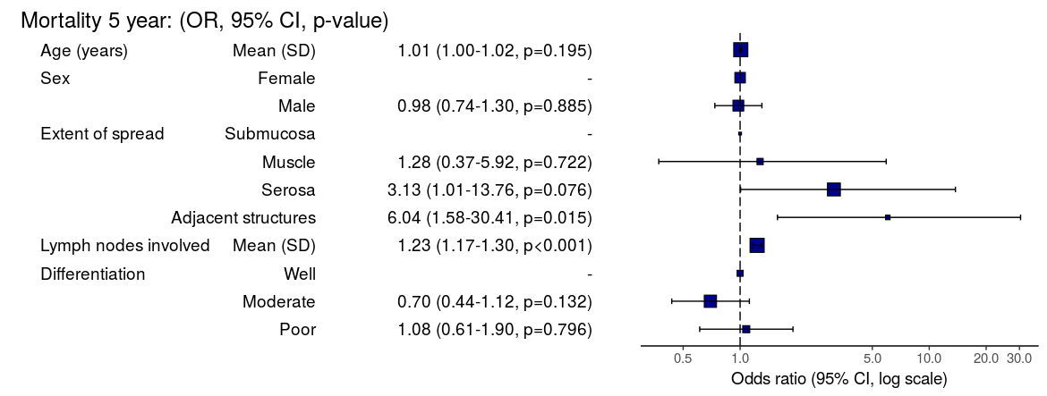
table2| Mortality 5 year | Alive | Died | OR (univariable) | OR (multivariable) | |
|---|---|---|---|---|---|
| Age (years) | Mean (SD) | 59.8 (11.4) | 59.9 (12.5) | 1.00 (0.99-1.01, p=0.986) | 1.01 (1.00-1.02, p=0.195) |
| Sex | Female | 243 (55.6) | 194 (44.4) | - | - |
| Male | 268 (56.1) | 210 (43.9) | 0.98 (0.76-1.27, p=0.889) | 0.98 (0.74-1.30, p=0.885) | |
| Extent of spread | Submucosa | 16 (80.0) | 4 (20.0) | - | - |
| Muscle | 78 (75.7) | 25 (24.3) | 1.28 (0.42-4.79, p=0.681) | 1.28 (0.37-5.92, p=0.722) | |
| Serosa | 401 (53.5) | 349 (46.5) | 3.48 (1.26-12.24, p=0.027) | 3.13 (1.01-13.76, p=0.076) | |
| Adjacent structures | 16 (38.1) | 26 (61.9) | 6.50 (1.98-25.93, p=0.004) | 6.04 (1.58-30.41, p=0.015) | |
| nodes | Mean (SD) | 2.7 (2.4) | 4.9 (4.4) | 1.24 (1.18-1.30, p<0.001) | 1.23 (1.17-1.30, p<0.001) |
| Differentiation | Well | 52 (56.5) | 40 (43.5) | - | - |
| Moderate | 382 (58.7) | 269 (41.3) | 0.92 (0.59-1.43, p=0.694) | 0.70 (0.44-1.12, p=0.132) | |
| Poor | 63 (42.3) | 86 (57.7) | 1.77 (1.05-3.01, p=0.032) | 1.08 (0.61-1.90, p=0.796) |
MS Word via knitr/R Markdown
Important. In most R Markdown set-ups, environment objects require to be saved and loaded to R Markdown document.
# Save objects for knitr/markdown
save(table1, table2, dependent, explanatory, file = "out.rda")
We use RStudio Server Pro set-up on Ubuntu. But these instructions should work fine for most/all RStudio/Markdown default set-ups.
In RStudio, select File > New File > R Markdown.
A useful template file is produced by default. Try hitting knit to Word on the knitr button at the top of the .Rmd script window.
Now paste this into the file:
---
title: "Example knitr/R Markdown document"
author: "Ewen Harrison"
date: "22/5/2018"
output:
  word_document: default
---
```{r setup, include=FALSE}
# Load data into global environment.
library(finalfit)
library(dplyr)
library(knitr)
load("out.rda")
```

## Table 1 - Demographics
```{r table1, echo = FALSE, results='asis'}
kable(table1, row.names=FALSE, align=c("l", "l", "r", "r", "r", "r"))
```

## Table 2 - Association between tumour factors and 5 year mortality
```{r table2, echo = FALSE, results='asis'}
kable(table2, row.names=FALSE, align=c("l", "l", "r", "r", "r", "r"))
```

## Figure 1 - Association between tumour factors and 5 year mortality
```{r figure1, echo = FALSE}
colon_s %>%
  or_plot(dependent, explanatory)
Create Word template file
Now, edit your Word file to create a new template. Click on a table.
The style should be compact. Right click > Modify… >
font size = 9. Alter heading and text styles in the same way as desired.
Save this as template.docx. Upload the file to your project
folder. Add this reference to the .Rmd YAML heading, as below. Make sure
you get the spacing correct.
The plot also doesn’t look quite right and it prints with warning messages. Experiment with fig.width to get it looking right.
Now paste this into your .Rmd file and run:
---
title: "Example knitr/R Markdown document"
author: "Ewen Harrison"
date: "21/5/2018"
output:
  word_document:
    reference_docx: template.docx
---
```{r setup, include=FALSE}
# Load data into global environment.
library(finalfit)
library(dplyr)
library(knitr)
load("out.rda")
```

## Table 1 - Demographics
```{r table1, echo = FALSE, results='asis'}
kable(table1, row.names=FALSE, align=c("l", "l", "r", "r", "r", "r"))
```

## Table 2 - Association between tumour factors and 5 year mortality
```{r table2, echo = FALSE, results='asis'}
kable(table2, row.names=FALSE, align=c("l", "l", "r", "r", "r", "r"))
```

## Figure 1 - Association between tumour factors and 5 year mortality
```{r figure1, echo = FALSE, warning=FALSE, message=FALSE, fig.width=10}
colon_s %>%
  or_plot(dependent, explanatory)
```
This is now looking good, and further tweaks can be made if you wish.
PDF via knitr/R Markdown
Default settings for PDF:
---
title: "Example knitr/R Markdown document"
author: "Ewen Harrison"
date: "21/5/2018"
output:
  pdf_document: default
---
```{r setup, include=FALSE}
# Load data into global environment.
library(finalfit)
library(dplyr)
library(knitr)
load("out.rda")
```

## Table 1 - Demographics
```{r table1, echo = FALSE, results='asis'}
kable(table1, row.names=FALSE, align=c("l", "l", "r", "r", "r", "r"))
```

## Table 2 - Association between tumour factors and 5 year mortality
```{r table2, echo = FALSE, results='asis'}
kable(table2, row.names=FALSE, align=c("l", "l", "r", "r", "r", "r"))
```

## Figure 1 - Association between tumour factors and 5 year mortality
```{r figure1, echo = FALSE}
colon_s %>%
  or_plot(dependent, explanatory)
```
Again, this is not bad, but has issues.
We can fix the plot in exactly the same way. But the table is off the side of the page. For this we use the ’kableExtra` package. Install this in the normal manner. You may also want to alter the margins of your page using geometry in the preamble.
---
title: "Example knitr/R Markdown document"
author: "Ewen Harrison"
date: "21/5/2018"
output:
  pdf_document: default
geometry: margin=0.75in
---
```{r setup, include=FALSE}
# Load data into global environment.
library(finalfit)
library(dplyr)
library(knitr)
library(kableExtra)
load("out.rda")
```

## Table 1 - Demographics
```{r table1, echo = FALSE, results='asis'}
kable(table1, row.names=FALSE, align=c("l", "l", "r", "r", "r", "r"),
                        booktabs=TRUE)
```

## Table 2 - Association between tumour factors and 5 year mortality
```{r table2, echo = FALSE, results='asis'}
kable(table2, row.names=FALSE, align=c("l", "l", "r", "r", "r", "r"),
            booktabs=TRUE) %>%
    kable_styling(font_size=8)
```

## Figure 1 - Association between tumour factors and 5 year mortality
```{r figure1, echo = FALSE, warning=FALSE, message=FALSE, fig.width=10}
colon_s %>%
  or_plot(dependent, explanatory)
This is now looking pretty good for me as well.
There you have it. A pretty quick workflow to get final results into Word and a PDF.